Contents

Page updated: October 13, 2021
Author: Curtis Mobley
View PDF

Dispersion

This page now reverts to the customary $k$ for the real wavenumber, $k = 2 π ∕ λ$ . The preceding page discussed wave propagation for a sinusoidal wave with given spatial ( $k$ ) and temporal ( $ω$ ) frequencies. In that case, there is a single speed of propagation, the phase speed $v_{p} = ω ∕ k$ . However a true sinusoidal wave cannot exist in nature because real waves must start and stop at ﬁnite times. This in turn means that the ﬁnite length “wave packet” must contain more than one frequency. (This is easily seen using Fourier transforms. The Fourier transform of a ﬁnite-length spatial function contains all frequencies.) It is then possible that the overall wave packet or group of waves propagates at a diﬀerent speed, called the group speed, than the phase speeds of the individual waves comprising the wave packet. This results in some waves “outrunning” others, and the original group of waves spreads out, or disperses.

This page examines dispersion in detail. The basic phenomenon of dispersion and diﬀerent phase and group speeds is illustrated ﬁrst by the sum of just two sinusoids. This is then generalized to wave packets containing all frequencies. This allows for an understanding of “normal” and “anomalous” dispersion. A speciﬁc example of phase and group speeds is then given for light wave propagation in pure water, which leads to a surprise.

Phase and Group Speeds for a Two-wave System

Let $ψ$ be the magnitude of a propagating disturbance. $ψ$ might be the electric ﬁeld of a light wave, or the height of the sea surface relative to the mean sea surface, or the ﬂuctuating pressure of a sound wave. Suppose that $ψ$ is composed of two cosines of equal amplitudes but diﬀering wave numbers and temporal frequencies. That is to say

ψ (x, t) = A cos (k_{1} x - ω_{1} t) + A cos (k_{2} x - ω_{2} t) .

(1)

The trigonometric identity

cos α + cos β = 2 cos (\frac{α - β}{2}) cos (\frac{α + β}{2})

can be used to rewrite $ψ$ as

ψ (x, t) = 2 A cos [\frac{1}{2} (Δ k x - Δ ω t)] cos (\bar{k} x - \bar{ω} t),

where $Δ k = k_{2} - k_{1}$ , $Δ ω = ω_{2} - ω_{1}$ , $\bar{k} = \frac{1}{2} (k_{1} + k_{2})$ , and $\bar{ω} = \frac{1}{2} (ω_{1} + ω_{2})$ . This can be rewritten as

ψ (x, t) = 2 A cos [\frac{1}{2} Δ k (x - \frac{Δ ω}{Δ k} t)] cos [\bar{k} (x - \frac{\bar{ω}}{\bar{k}} t)]

Recalling that a function of the form $f [s (x - v t)]$ propagates with speed $v$ , we see that the two cosines describe waves that propagate with two speeds,

ψ (x, t) = 2 A cos [\frac{1}{2} Δ k (x - v_{g} t)] cos [\bar{k} (x - v_{p} t)],

where we identify the two speeds as

\begin{align} v_{p} = & \frac{\bar{ω}}{\bar{k}}, a n d & (2) \\ v_{g} = & \frac{Δ ω}{Δ k} . & (3) \end{align}

$v_{p}$ has the form of the phase speed of the previous section, computed now from the average wave number and average angular frequency. $v_{g}$ is called the group speed and is computed as the ratio of the diﬀerences in the two wave numbers and frequencies.

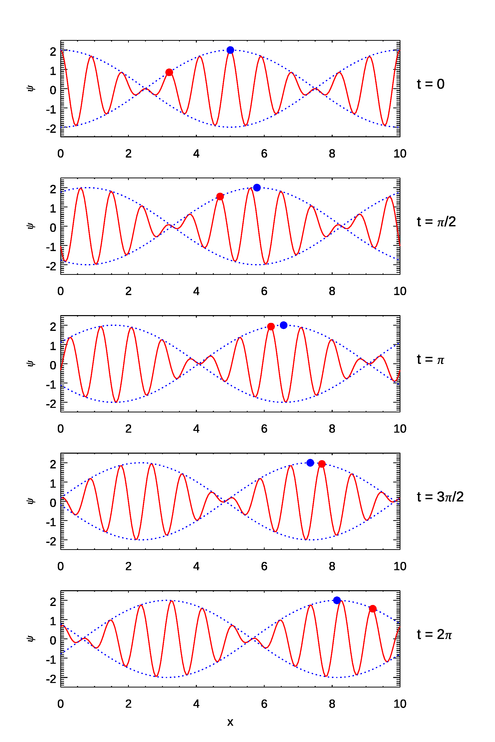
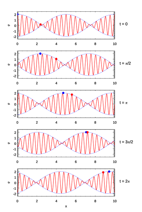
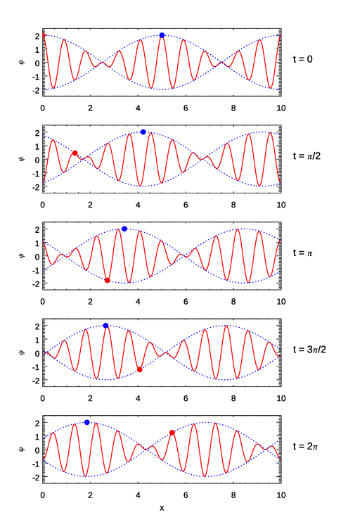
The implications of these equations are illustrated in Figs. 1–3. In the ﬁrst ﬁgure the wave numbers and frequencies are chosen so that both the individual waves (the red curves) and the group envelope (the blue dots) propagate in the same direction and $v_{p} > v_{g}$ . In the second ﬁgure the wave numbers and frequencies are chosen so that both the waves and the group envelope propagate in the same direction but with $v_{p} < v_{g}$ . In the third ﬁgure the wave numbers and frequencies are chosen so that the waves propagate in one direction but the group envelope propagates in the opposite direction.

Figure 1: Illustration of phase and group speeds for the two-wave system giving

v_{p} > v_{g}

. The blue dots track the crest of the wave envelope. The red dots track the crest of a particular wave phase that forms at the rear of an envelope and moves forward, growing in amplitude and eventually passing the crest of the envelope, after which it decreases in amplitude as it propagates further and eventually dies out. The parameter values used in Eq. (1) are

A = 1

ω_{1} = 2 π, ω_{2} = 1.1 ω_{1}

, and

k_{1} = 2 π, k_{2} = 1.2 k_{1}

. The resulting phase and group speeds are

v_{p} = 0.9545

and

v_{g} = 0.50

, so both waves propagate to the right in the ﬁgure but the individual waves outrun the wave packet.

Figure 2: Illustration of phase and group speeds for two waves giving

v_{p} < v_{g}

. As before, the blue dots track the crest of the wave envelope. The red dots track the crest of a particular wave phase that forms at the front of an envelope. Although the red dot moves to the right (

v_{p} > 0

), from the viewpoint of the wave packet, the wave forms at the front of the packet and moves to the rear of the packet, where it dies out. The parameter values used in Eq. (1) are

A = 1

ω_{1} = 4 π, ω_{2} = 1.15 ω_{1}

, and

k_{1} = 4 π, k_{2} = 1.1 k_{1}

. The resulting phase and group speeds are

v_{p} = 1.024

and

v_{g} = 1.50

, so now the individual waves propagate slower than the wave packet.

Figure 3: Illustration of phase and group speeds for two waves giving

v_{p} > 0

and

v_{g} < 0

. The blue dots track the crest of the wave envelope and the red dots track the crest of a particular wave phase. The parameter values used in Eq. (1) are

A = 1

ω_{1} = 2 π, ω_{2} = 0.9 ω_{1}

, and

k_{1} = 2 π, k_{2} = 1.2 k_{1}

. The resulting phase and group speeds are

v_{p} = 0.8636

and

v_{g} = - 0.50

. Now the individual waves propagate to the right, but the group envelope propagates to the left.

Dispersion Relations

We have seen that the phase speed is the ratio of angular frequency to wave number. It is easy to see from the previous example that if the two waves have nearly the same frequencies and wave numbers that $Δ ω ∕ Δ k$ is a good approximation to the derivative $d ω ∕ d k$ . In the general development below, the group speed will be deﬁned as

v_{g} = \frac{d ω}{d k} .

(4)

Clearly, knowing how $ω$ depends on $k$ allows the computation of both the phase speed and the group speed. This relation is known as a dispersion relation.

Do the situations illustrated in Figs. 1–3 actually occur in nature? Indeed they do. Consider waves propagating on a water surface. The dispersion relation for small amplitude, free-surface water waves is (e.g., Apel (1987))

ω^{2} = (g k + \frac{σ}{ρ} k^{3}) tanh (k h),

(5)

where $g = 9.8 m s^{- 2}$ is the acceleration of gravity, $σ = 0.074 N m^{- 1}$ is the surface tension of water, $ρ = 1000 k g m^{- 3}$ is the density of water, and $h$ is the depth of the water. [The assumption that the waves have a small amplitude allows the equations of ﬂuid motion to be linearized, which results in the dispersion relation shown here.]

This dispersion relation has three limiting cases of interest.

For waves whose wavelengths are small compared to the water depth, so-called deep-water waves, $tanh (k h) = tanh (2 π h ∕ λ) \approx 1$ . Then

ω^{2} = (g k + \frac{σ}{ρ} k^{3}) .

For long-wavelength “gravity waves”, $k > > k^{3}$ and the surface-tension term is negligible (i.e., surface tension is a negligible restoring force compared to gravity). Then

ω^{2} \approx g k .

From this we can compute $v_{p} = ω ∕ k = \sqrt{g ∕ k}$ and $v_{g} = d ω ∕ d k = \frac{1}{2} \sqrt{g ∕ k}$ . Thus the group speed for deep-water gravity waves is one-half the phase speed. For very short-wavelength capillary waves, $k$ is large and the surface-tension term dominates. Then

ω^{2} \approx \frac{σ}{ρ} k^{3},

from which we ﬁnd $v_{p} = \sqrt{σ k ∕ ρ}$ and $v_{g} = \frac{3}{2} \sqrt{σ k ∕ ρ}$ . Thus the group speed is $\frac{3}{2}$ times the phase speed. For wavelengths that are large compared to the water depth, so-called shallow-water waves, $tanh k h \approx k h$ and, again, the surface tension term is negligible. The dispersion relation is then

ω^{2} \approx g h k^{2},

from which we get $v_{p} = v_{g} = \sqrt{g h}$ . Thus for shallow-water waves the phase and group speeds are equal.

The deep-water case of $v_{g} = \frac{1}{2} v_{p}$ is qualitatively like Fig. 1. The individual waves travel faster than the group envelope. The individual waves appear to form at the back of the envelope, move forward to the crest of the envelope while growing in amplitude, and then move past the crest of the envelope and decrease in amplitude until they disappear at the front of the group. I have watched this happen many times while sea kayaking on a nearly calm water water body. Then a ship goes by some distance away and leaves a large wake composed of a string of smaller waves. As the wake reaches my kayak, smaller waves form at the rear of the wake group and propagate to the front of the wake, where they disappear. I never cease to be amazed as I watch waves appear from nowhere, grow in size as they propagate forward, and then simply disappear when they reach the front of the wake, exactly as predicted by the deep-water dispersion formula.

The capillary-wave case of $v_{g} = \frac{3}{2} v_{p}$ is similar to Fig. 2. The very short-wavelength capillary waves form at the front of the wave packet and propagate to the rear, or rather, the wave packet envelope outruns them. An example of a positive phase speed and a negative group speed will be seen below.

The General Development

This section merely outlines the general development of wave propagation in dispersive media; a more complete discussion is given in Section 7.3 of Jackson (1962) and in Sections 16-4 and 16-5 of Towne (1967). We have learned that a single sinusoidal wave of given frequency $ω$ and wave number $k$ satisﬁes the wave equation and has a wave propagation speed of $ω ∕ k$ . Because the wave equation is linear, a linear combination of sinusoids also satisﬁes the wave equation. Thus a general wave function $ψ (x, t)$ can be built up as a sum of sinusoids of various amplitudes, frequencies, and wave numbers. Rather than deal with real sinusoids as seen in Eq. (1), it is convenient (indeed, almost necessary) to use the complex representation of propagating waves. We thus write

\tilde{ψ} (x, t) = \int_{- \infty}^{\infty} \tilde{A} (k) exp i [k x - ω (k) t] d k,

(6)

where the tilde reminds us that the quantity is a complex function whose real value must be taken at the end of the development. Positive and negative $k$ values represent waves with the same physical wave number but traveling in opposite directions. This equation thus adds up waves of any amplitude and wavenumber to create a general waveform. Note that the angular frequency is a function of the wave number according to the dispersion relation for the medium under study. (It is also noted that at $t = 0$ this equation is, to within a factor of $2 π$ , precisely the inverse Fourier transform of $\tilde{A} (k)$ , although that connection will not be used here.)

The dispersion relation can be expanded in a power series about any value of $k_{o}$ :

ω (k) = ω_{o} + {\frac{d ω}{d k}|}_{o} (k - k_{o}) + h i g h e r o r d e r t e r m s .

(7)

If the distribution of $\tilde{A} (k)$ values is peaked around the value $k_{o}$ , or if the dependence of $ω$ on $k$ is weak, then the higher order terms can be neglected. Use of this approximation in Eq. (6) eventually leads to the identiﬁcation of $v_{g} = d ω ∕ d k$ as shown in (4) as the speed at which a wave pulse or packet travels. But note: as will be seen, neglecting the higher order terms in this expansion in not always a good approximation.

For light waves in a dielectric medium like water or glass the dispersion relation is

ω (k) = \frac{c k}{n (k)},

(8)

where $c$ is the speed of light in a vacuum and $n (k)$ is the real index of refraction expressed as a function of $k$ . This gives the phase speed as

v_{p} = \frac{ω}{k} = \frac{c}{n (k)} .

(9)

This make clear that “the speed of light in a medium” as presented in freshman physics is the phase speed. The corresponding group speed is

v_{g} = \frac{d ω}{d k} = \frac{d}{d k} [\frac{c k}{n (k)}] = \frac{c}{n (k)} - \frac{c k}{n {(k)}^{2}} \frac{d n (k)}{d k} .

It is more convenient to view the index of refraction as a function of frequency than of wave number, so using

\frac{d n}{d k} = \frac{d n}{d ω} \frac{d ω}{d k} = (\frac{c}{n} - \frac{c k}{n^{2}}) \frac{d n}{d ω}

in the previous equation leads to

v_{g} = \frac{c}{n (ω) + ω \frac{d n (ω)}{d ω}} .

This is the form usually seen in physics texts. The corresponding equation with $n$ viewed as a function of wavelength (as oceanographers prefer to do) is

v_{g} = \frac{c}{n (λ)} (1 - \frac{λ}{n (λ)} \frac{d n (λ)}{d λ}) = v_{p} (1 - \frac{λ}{n (λ)} \frac{d n (λ)}{d λ}) .

(10)

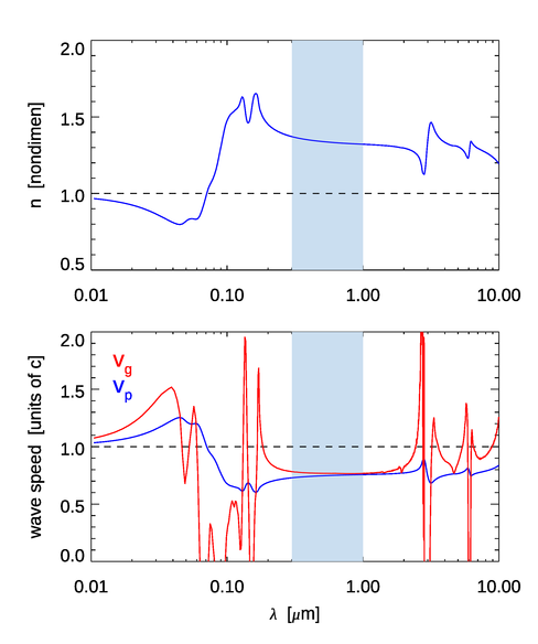
Note that if $n$ is independent of wavelength, $v_{g} = v_{p}$ . This is approximately the case for water at wavelengths near 1000 nm, as seen in the top panel of Fig. 4. If $n = 1$ , $v_{g} = v_{p} = c$ . The only “substance” with $n = 1$ is a vacuum.

It is very instructive to examine these phase and group speeds when applied to the propagation of light in pure water. The top panel of Fig. 4 shows the real index of refraction of pure water for $λ = 0.1$ – $10 μ m$ . The bottom panel shows the corresponding phase and group speeds computed from Eqs. (9) and (10), respectively. There are a number of features to note in these curves. Below 72 nm, the real index of refraction is less than 1, which makes the phase speed $v_{p} = c ∕ n$ greather than $c$ . This is not a violation of special relativity. The “universal speed limit” of $c$ applies to material objects and the speed at which energy or signals can propagate; phase speeds can have any value. Between about 200 and 2000 nm, which includes the region of interest to optical oceanographers, $n (λ)$ decreases smoothly with increasing wavelength. The group speed is a bit greater than the phase speed, and both are about three-fourths the speed of light in a vacuum. However, there are regions where the group speed displays a seemingly bizarre behavior—it can be greater than the speed of light, and it can be negative, and there are rapid ﬂuctuations between these two extremes. The conventional wisdom of undergraduate physics says that energy propagates at the group speed, which therefore should not exceed the speed of light in vacuo.

What is happening here is that the concept of the group speed of a wave packet has broken down. Note in the ﬁgure that the large ﬂuctuations in $v_{g}$ occur near the wavelengths where $n (λ)$ is changing rapidly. Rapid changes in the index of refraction give rapid changes in the dispersion relation of Eq. 8. This in turn means that the higher order terms in the expansion of $ω (k)$ seen in Eq. (7) cannot be neglected. When that is the case, the simple concept of a group speed as deﬁned by Eq. (4) is inadequate to describe the propagation of the wave pulse envelope. As the venerable Jackson (1962) points out (on his page 211), a value of $v_{g} > c$ “...is no cause for alarm that our ideas of special relativity are here violated; group velocity is no longer a meaningful concept.” and “The behavior of the pulse is much more involved.” Towne (1967) (Section 6-5) and Bohren and Huﬀman (1983) (Section 9.1.3) discuss the physical processes leading to $n < 1$ . It is true for all substances that at high frequencies (short wavelengths) $n$ approaches 1 from values less than 1, just as is seen for water in Fig. 4.

Figure 4: Phase and group speeds for water. The top panel shows the real index of refraction of pure water (data of Segelstein (1981) redrawn from Fig. 1 of the water IOPs page). The bottom panel shows the phase speed

v_{p}

computed using Eq. (9) (blue curve) and and the group speed

v_{g}

computed from Eq. (10) (red curve). The black dashed line is the speed of light. The region of interest to optical oceanography, 300-1000 nm, is shaded in blue.

Dispersion

Phase and Group Speeds for a Two-wave System

Dispersion Relations

The General Development

Comments for Dispersion: